Business Statistics: Data Handling with Excel
In this tutorial, you will learn the following:
- Introduction of Data Types
- Mean, mode, range and quartiles
- Standard Deviation - both for samples and populations
- How to use basic Excel functions for statistical data analysis
- How to use advanced Excel functions for statistical data analysis
- How to use PivotTables for statistical data analysis.
- You will be given an Excel data sheet to download and use for free
- How to validate data with Excel Data Validation tools
- COUNTIF, SUMIF, LOOKUP,INDEX, AVERAGE, MEDIAN, MODE functions
- Correlation and Pearson's Product Moment Correlation Coefficient - PMCC
- Regression Line and Forecasting - LINEST AND FORECAST functions
- Spearman's Rank
- Normal Distribution
- Z-Scores
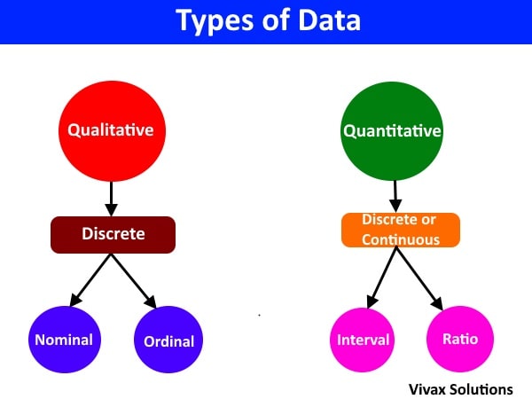
Data Types
The two major types of data that we encounter in our daily lives are:
- Qualitative Data
- Quantitative Data
Qualitative Data
The data is in the form of a description and not countable.
E.g. Hair colour, religion, race
Qualitative data is discrete, because the data points are well positioned with nothing in between.
Quantitative Data
The data is in the form of numbers.
E.g. Height, size of the foot, temperature, humidity
Quantitative data can either be continuous or discrete
E.g. Shoe size - discrete; size of the foot - continuous
Qualitative data is of two types:
- Nominal - referring to categories such as gender, race, religion etc.
- Ordinal - referring to order such as [hot, cold, cool, freezing],[1st, 2nd, 3rd]
Quantitative data is of two types:
- Interval - data points occur at regular intervals and zero exists and significant - Celsius temperature scale.
- Ratio - data points can occur at any order and zero means non-existence - weight, height, length etc
The following summarizes the above:
Now, let's look at the following paragraph and identify the data types by the colour.
The legendary climber, divided aspiring climbers into two groups, based on the individual gender, before embarking on the expedition. Each climber was handed down a thermometer, depending on the familiarity with the scale - Celsius or Fahrenheit. Each climber must note the altitude in their notebooks every hour. In addition, steepness of the climb must be declared in terms of moderate, steep and extremely steep, after every 15 minutes. After main meals of the day, they must record the weight of their backpacks.
🔑
Nominal
Interval
Ratio
Ordinal
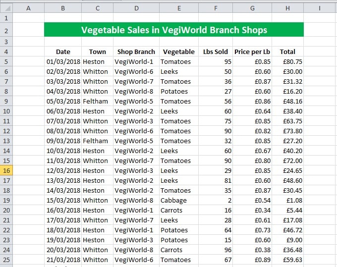
Throughout this tutorial, the following Excel datasheet will be used for analysis.
It is based on a fictional vegetable store chain, VegiWorld, based in West London, UK. It has several branches in three towns and in the dataset, the type of vegetable, its sales, the store name, and the town are displayed.
The data has been collected for a period of 45 days.
A section of the data sheet is shown below:
You can download the complete Excel datasheet by clicking here.
Location: mean, median and mode
Mean = sum of data / number of data
E.g.2, 3, 4, 5, 6
mean = (2 + 3 + 4 + 5 + 6) / 5 = 4
Median - the middle number when data is in order of size
E.g.1,3,2,5,4
Rearrangement: 1, 2, 3, 4, 5
Middle value, (n+1)th/2 value = 3rd value = 3
2, 5, 6, 4, 8, 12
Middle value, (n+1)th/2 value = 3.5th value = (6 + 4)/2 = 5
Mode - the value that occurs most
E.g.3, 4, 5, 6, 8, 9, 6
Mode = 6
E.g.3, 4, 5, 6, 8, 9, 6, 8, 8
Mode = 6, 8
Spread: range, IQR, standard deviation
Range - the difference between the maximum and minimum value of a data set
E.g. 2, 4, 5, 7, 18
Range = 18 - 2 = 16
E.g. 5, 2, 3, 10, 6
Range = 10 - 2 = 8
IQR = the difference between the third quartile and the first quartile = Q3 - Q1
E.g. 4, 7, 4, 5, 6, 2, 8
Place them order first: 2, 4, 4, 5, 6, 7, 8
Q1 = 4
Q3 = 7
IQR = Q3 - Q1 = 3
Standard Deviation: - the mean deviation from the mean = √Σ(x - x̄)2/n
E.g.2, 3, 4, 6, 10
x̄ = Σx/n = (2 + 3 + 4 + 6 + 10)/5 = 5
Σ(x - x̄)2/n = ((2 - 5)2 + (3 - 5)2 + (4 - 5)2 + (6 - 5)2 + (10 - 5)2)/5
= 8
Standard deviation = σ = √8 = 2.8
Location and Spread of Data - interactive practice
With the following applet, you can practise the calculations of the values of averages and spread of a given dataset. CLick the button to generate new datasets.
Standard Deviation - the concept and its need in data analysis
Consider the following data about the heights of plants in Jonathan's garden:
3cm, 4cm, 5cm, 7cm, 11cm
Now, let's calculate the mean - μ - of these values.
μ = (3 + 4 + 5 + 7 + 11)/5 = 6cm
If we use this value to describe the mean height of plants,
we immediately run into difficulties; because, it does not represent the true nature of heights of these plants - some are as
short as 3 cm and some are as tall as 11 cm.
Therefore, the mean in this case, to say the least, is a bit misleading. This leads to a need of another value that helps us to understand the distribution
of data in a given situation.
Now let's see how much each value of data has deviated ( going away ) from the
mean:
| x | 3 | 4 | 5 | 7 | 11 |
|---|
| μ | 6 | 6 | 6 | 6 | 6 |
|---|
| (x - μ) | -3 | -2 | -1 | 1 | 5 |
|---|
Let's find the average of these deviations from the mean value:
Σ(x - μ) / 5 = (-3 + -2 + -1 + 1 + 5 )/5 = 0
The deviations turned out to be zero, not because of lack of deviations; it is because, the deviations turned out to be
negative and positive which in the end led to be cancelled out.
Now, in order to deal with issue, let's square the deviations to remove the negative signs, which is as follows:
| x | 3 | 4 | 5 | 7 | 11 |
|---|
| μ | 6 | 6 | 6 | 6 | 6 |
|---|
| (x - μ) | -3 | -2 | -1 | 1 | 5 |
|---|
| (x - μ)2 | 9 | 4 | 1 | 1 | 25 |
|---|
Since we squared the deviations, just to deal with negative values, it's time we
reversed the process: let's find the square root of the following result:
√(Σ(x - μ)2)/5 = √(40/5) = 2.8
This is called the standard deviation of the above set of
data representing the heights of plants in Jonathan's garden. It gives us a clearer picture of data
distribution along with the mean. With the value of the standard deviation, the data can be described
in the following way:
The mean height of the plants in Jonathan's garden is 6cm and the standard deviation is 2. 8. That means the heights of most plants falls into the range from (6-2.8) = 3.2cm to (6+2.8)=8.8cm.
The example shows how important the Standard deviation is to get a clear picture about a set of data. Without it, talking about data is like, recalling the
fate of Titanic without the iceberg!!
So, the formula for standard deviation is as follows:
σ = √Σ(x - μ)2/N
where N is the total frequency.
Calculator-friendly formula for Standard Deviation
σ = √(Σ(x - μ)2)/N
σ = √(Σ(x2 - 2xμ + μ2)/N
σ = √(Σ(x2 - Σ2xμ + Σμ2)/N
σ = √(Σ(x2 - 2μΣx + Σμ2)/N
σ = √(Σ(x2 - 2μnμ + nμ2)/N
σ = √(Σ(x2 - 2nμ2 + nμ2)/N
σ = √(Σ(x2 - nμ2)/N
σ = √(Σx2/N) - μ2
σ = √(Σx2/N) - μ2
To find the standard deviation in grouped data, we change the method
slightly - σ = √(Σf(x - μ)2)/N, where f is the frequency of each
class and N is the total frequency.
E.g.
The frequency of shoe sizes of students in a certain class is as follows:
| shoe-size(x) | frequency(f) |
|---|
| 3 | 3 |
| 4 | 5 |
| 5 | 10 |
| 6 | 8 |
| 7 | 4 |
μ = Σfx/N = 5.2
σ = √(Σf(x - μ)2)/N = √(Σf(x - 5.2;)2)/30 = 2.3
E.g.
The marks obtained by a group of students for maths are as follows:
| Marks(x) | frequency(f) |
|---|
| 0 - 20 | 3 |
| 21 - 40 | 6 |
| 41 - 60 | 9 |
| 61 - 80 | 8 |
| 81 - 100 | 4 |
μ = Σfx/N = 52.7
σ = √(Σf(x - μ)2)/N = √(Σf(x - 52.7)2)/30 = 2.55
I am sure, you have got a good understanding of the concept of standard deviation by now.
Population and Sample Parameters
In statistics, it's in the population where real data lies; however, its sheer size, such as the fish in a lake or number of rabbits in a game reserve, may make us finding them next to impossible. In these circumstances, we take samples - manageable sections of the population, assuming they fairly represent the population - in order to estimate the corresponding parameters of the population. These values are sample parameters.
Once sample parameters are found, further statistical tests must be carried out to make them realistically closer to the corresponding population values.
E.g.
In order to find the sample standard deviation, Sn-1, the formula is edited as follows:
Sn-1 = √Σ(x - x̄)2/n-1
The division by n-1, instead of n, as calculations show, brings the sample standard deviation closer to that of the population. The method of finding the sample mean remains the same, though.
x̄ = Σx/n
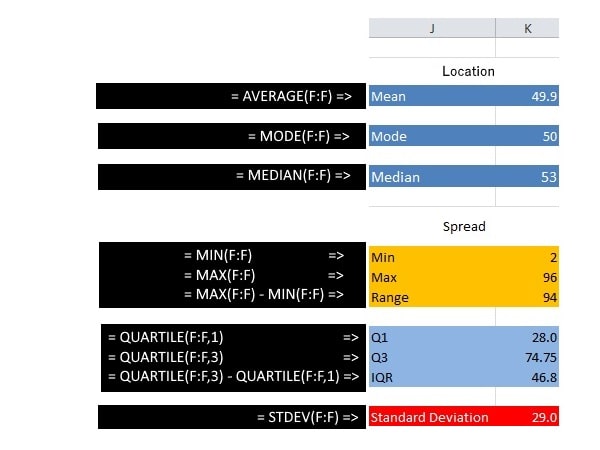
Using Excel functions to find location and spread of data
Excel has built-in functions to perform all the tasks easily. This is how it appears, when done.
For this exercise, the weight of vegetables field, Column F is used. The range is described as F:F in all Excel functions.
Using advanced Excel functions to analyse data
In this section, the Excel datasheet is analysed by advanced functions of Excel. They are as follows:
- COUNTIF() function
- COUNITIFS() function with multiple criteria
- SUMIF() function
- SUMIFS() function with multiple criteria
- INDEX() function combined with MATCH() function
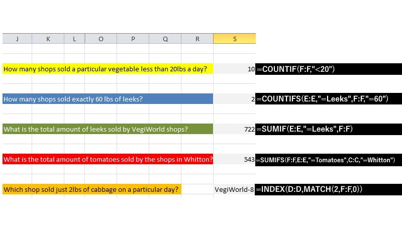
The functions are self-explanatory as they are given next to the output expected of them.
PivotTables
A PivotTable is a special tool in Excel that can perform the above tasks that we normally do with the aid of built-in functions. With a PivotTable, Excel can calculate, summarize, and analyze data in order to trends and patterns.
In order to create a PivotTable, please follow the steps below:
- Click anywhere in the Excel sheet.
- Click the Insert tab Menubar.
- Now, click the PivotTable icon on the icon bar.
- Choose the default settings and click OK.
- The PivotTable will be created in a new sheet by default. Look at the bottom of the datasheet and choose the new addition.
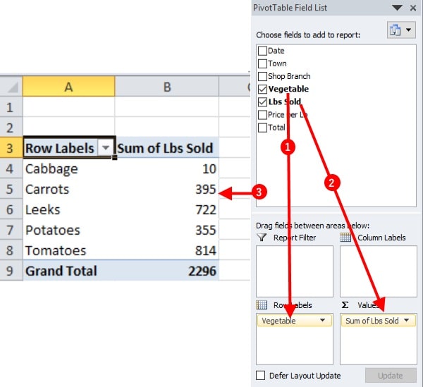
Task 1: Finding the amount of vegetables sold in lbs
- Drag down the Vegetable field from the top container and drop under Row Labels.
- Drag down the Lbs Sold field from the same and drop under Σ Values
You will see the data now exactly the way you want them to in.
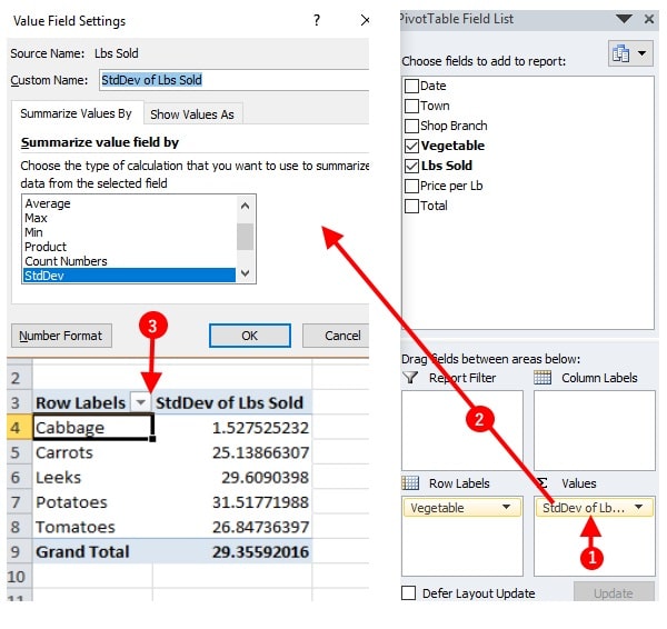
Task 2: Finding mean and standard deviation of vegetables sold
- Drag down the Vegetable field from the top container and drop under Row Labels.
- Drag down the Lbs Sold field from the same and drop under Σ Values
- Now click the button under Σ Values and then click Value Field Settings tab.
- Choose from the options - Sum, STDEV, AVERAGE - and see the PIVOTTABLE being updated instantly.
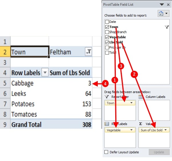
Task 3: Finding the amount of vegetables sold based on the town
- Drag down the Vegetable field from the top container and drop under Row Labels.
- Drag down the Lbs Sold field from the same and drop under Σ Values
- Drag down the Town field in the Report Filter container
- Now, a PivotTable with a filter can be created. Choose a town from a filter to see the relevant data for the town.
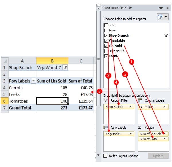
Task 4: Finding the amount of vegetables sold and earnings based on the shop
- Drag down the Vegetable field from the top container and drop under Row Labels.
- Drag down the Lbs Sold field from the same and drop under Σ Values
- Drag down the Shop Branch field in the Report Filter container
- Drag down the Total field and drop under Σ Values; you can move it up or down with the mouse.
- Now, a PivotTable with a filter and three columns can be created. Choose a shop from a filter to see the relevant data for the shop.
Data Analysis - LOOKUP() function
In this example, Excel LOOKUP() function that takes three parameters is used on a plain set of data. The best way to understand the function
is going through an example, rather than the focussing on the parameters taken in by the function.
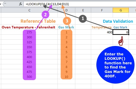
In the preceding example, the table on the left is the Gas Mark against Oven Temperature in Fahrenheit.. This is usually the reference table in data validation.
On the right of the diagram lies, the actual data to be analysed. If the temperature is given, we use Excel LOOKUP() function to find out the corresponding Gas Mark.
The contents - parameters - of the LOOKUP functions are as follows:
LOOKUP(value to be analysed, values in the reference table, the column where the result comes from)
For example, I want to find out the Gas Mark for 4000F. The image shows how it is done. The result will be 6.
Data Validation - drop down lists
Excel data validation tools can be used to create drop down lists to take data from to fill up cells with data.
- Select the cell, just below Temperature in Fahrenheit.
- Choose Data on the Home tab and then select Data Validation.
- Choose List from the drop down list under Allow.
- Undersource, type in the temperatures with a comma as the separation - 275,300,325,350,375,400,425,450,475,500.
- Repeat the same for Gas Mark, by selecting the cell under it - 1,2,3,4,5,6,7,8,9,10
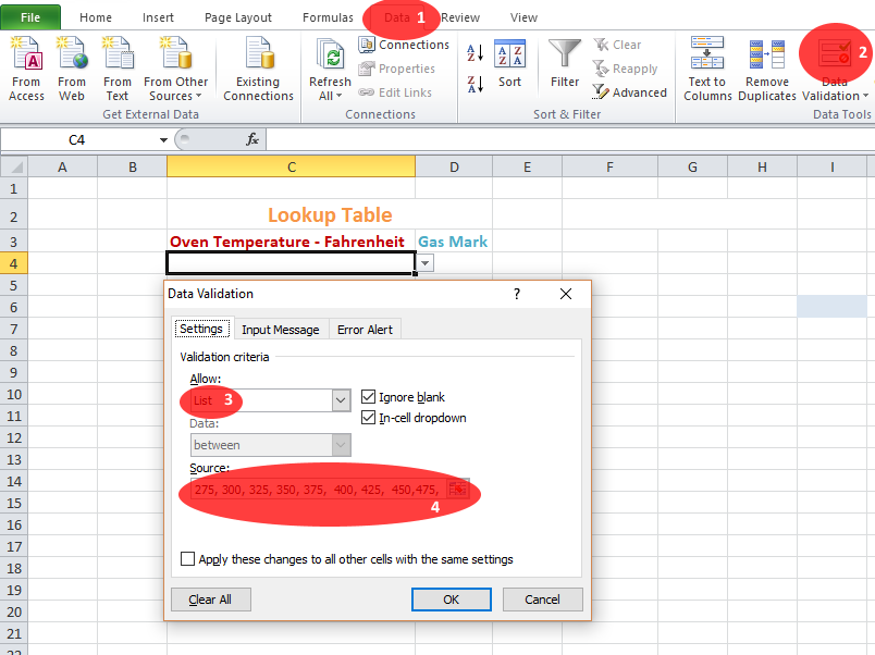
Once done, the Excel worksheets looks like this:
Correlation
The relationship between two quantitive variables is known as correlation.
The correlations can be:
- Positive Correlation - an increase in one variable leads to an increase in the other
- Negative Correlation - an increase in one variable leads to a decrease in the other
- No Correlation - the increase or decrease in one variable is not related to the other
The following spreadsheet shows three sets of data and the corresponding scatter diagrams.
The correlation can be quantified by Pearson's Product Moment Correlation Coefficient, PMSS - r. It's value ranges from -1 to 1.. A value of zero or close to zero indicates the absence of any correlation between the two sets of data. On the other hand, if it is close to 1, it's a strong positive correlation; if it's close to -1, it's a negative correlation.
To find Sxy, add the values in the cells, E43:E49. In order to find, Sxx and Syy, please add the values in the cells, C43:C49 and D43:D49 respectively.
Regression Line and Forecasting
Once a set of data is plotted and a scatter diagram is produced, the trendline can be drawn easily. In Excel, just right-click any data point on the grid and choose add trendline option. By default, linear option is selected. You can choose the equation of the trendline too.
Since the line is a straight line, it is in the form of y = b + ax, where a and b are the gradient and intercept of the line respectively.
In order to find, a and b in Excel, follow the steps below:
- Select a cell and enter = LINEST(Y-range, X-range, TRUE, FALSE)
- Select the adjacent horizontal cell and enter = LINEST(Y-range, X-range, TRUE, FALSE) again.
- Select the two cells and press F2.
- Select the two cells and press Ctrl, Shift and Enter together.
With the above steps, you can find a and b.
Since we know the equation of the regression line, a and b, we can use it to forecast the data, if one of the variable is known. In Excel, we use FORECAST(data value, y-range, x-range) to predict the values.
Interpolation
If the data value is in the known range, in this case 70C, we can predict the corresponding Gas bill - interpolation.
Extrapolation
If the data value is outside the known range, in this case 130C, we still can predict the corresponding Gas bill - extrapolation.
Spearman's Rank
We have seen how the concept of correlation is utilized, when it is associated with the relationship between two quantitive variables. For example,
the number of fans sold by a superstore with the rise of humidity during a summer
period is a case in point.
| Average Relative Humidity(%) |
Fans Sold |
| 29 |
1200 |
| 32 |
1280 |
| 45 |
2200 |
| 65 |
3400 |
| 75 |
3800 |
In the above example, we can
quantify the variables involved - they take numbers. So, we plot a graph of the
two variables to see a relationship between the two and they go a step further
to justify it in a mathematical manner to make it statistically
appealing. In short, there is clearly a strong relationship between the two variables, the relative humidity and the sales of fans.
Some variables cannot be
represented by numbers, though. yet, they can be arranged in a certain order so
that the pattern makes sense to those who are interested in them.
This is what led Charles Edward Spearman, the British psychologist, to coming up with a method to rank the variables first and then find the correlation coefficient between the ranks, which came to be known as Spearman's Rank.
It's something best learned by following a real-life example, which is as follows:
E.g.
Suppose there is a beauty contest involving ten aspiring models and the enviable job of choosing the winner is in the hands of two judges.
Since beauty cannot be
quantified, the judges have to rank them, say, 1 - 10, by taking into account a few factors, usually associated with beauty pageants.
Spearman's Rank(ρ), exactly like Pearson's Correlation Coefficient, can take any value between -1 and +1, indicating a strong negative correlation and a strong positive correlation respectively. If it's zero, there is no correlation between the ranks of the variables involved.
In the above example, ρ = 0.89. So, there is a strong correlation between the ranks given by Judge A and Judge B, in determining the beauty of the contestants of the pageant.
Here is an opportunity for you to practise Spearman's Rank interactively.
E.g.
Some bottles of wine can be
arranged by the responses to their taste. The arrangement makes sense to people
who are fond of wine, despite the absence of an index to measure it.
In these circumstances,
Spearman's rank comes to our rescue. It can easily be used to determine the
relationship between the two variables without numbers, but with ranks. Since it is universally
accepted as a trusted method, we can easily cash in on this encouragingly simple
method.
Since we do not have numbers
for the variable, we assign numbers to them, in a sensible way. They are
called ranks.
E.g.
Suppose there are five wine bottles A,
B, C, D and E in the order of taste. We can assign ranks to them in the order of
5,4,3,2,1 or 10, 8.6, 4,2 . These are arbitrary values assigned to variables in
a sensible way; there are not hard and fast rules about it. However, the simpler
the better.
The ranking system must be
extended to both sets of variables. Then a formula must be used to find
Spearman's rank, the value of which determines the correlation.
| Ranks of variable X | Ranks of variable Y | Ranks of variable X - Ranks of variable Y |
| x1 |
y1 |
d1 |
| x2 |
y2 |
d2 |
| x3 |
y3 |
d3 |
Spearman's rank (rs) = 1 -
6∑d2 / [n(n2-1)]
The value of lies between o and 1 (inclusive)
Now, you can use the above data in the following calculator in order to find Spearman's Rank.
We can find the Spearman's Rank for quantitive data as well. The data, however, must be ranked exactly like we did it with qualitative data in the previous example first, though.
In order to rank the data, the smallest data value was given rank 1, the next value, rank 2 etc.
Normal Distribution
Frequencies of most of the well-known measurements related to human beings, when plotted against the latter
take the following form for large amount of data. The measurements in question are said to be normally distributed.
The above frequency distributions - and many similar ones - have the following properties:
- They are symmetrical around a mean value.
- The frequency approaches zero for very large value of the variable on both sides.
- The curve is bell-shaped.
- Mean, mode and the median are the same.
If the frequency is turned into probability - dividing it by the total frequency - the shape still remains the same. It's then called the Normal Distribution curve. So, the total area under the curve is 1. Three Normal Distributions are shown as follows:
N ~ (μ, σ2); μ = mean, σ = standard deviation
With the following applet, you can choose the mean and the standard deviation of the Normal Distributions and then explore how the probability changes.
Please use the following steps in order to calculate the probabilities.
- Choose your mean and standard deviations.
- Choose the region where you need the probability of.
- Adjust the sliders to find the probabilities you need.
Standard Normal Distribution - Z-Score
Since there are thousands of real life situations to be modelled by the Normal Distribution, there are equal number of mean and standard deviation values to go with them.
This poses a significant challenge when it comes to calculations. Of course, there are calculators, as given above, which can deal with it. Before they came into being, however, this was somewhat problematic, because maintaining tables was the only option left.
In order to address this issue, statisticians came up with standardizing the Normal Distributions in such a way that a single table could solve the problem. The Standard Normal Distribution is defined as follows:
Z ~ (0, 12)
In the Standard Normal Distribution, the mean and the standard deviation are 0 and 1 respectively. It's a hypothetical distribution.
In order to change a variable in the Normal Distribution, x, to that of the Standard Normal Distribution, the following step is used.
Z = (X -μ)/σ, Z is called, Z-Score.
Once this is done, the single table available for the standard normal distribution can be used for calculations.
E.g.
Batteries for a portable radio have a mean life of 120 hours and a standard deviation of 15. Assuming that the battery life is normally distributed, find the proportion of batteries with mean life between 130 and 150. Find the proportion of batteries that lie within a range of 80%, around the mean.
X ~ (120, 152) => Z ~ (0, 12)
1)
Turning into the standard variable, Z = (X - 120)/15
p(130 < X <150) = P(10/15 < Z < 30/15) = P(2/3 < Z < 2)
If you adjust the above applet with μ = 0 and &sigma and move the sliders, you will see,
P(2/3 < Z < 2) = P(Z < 2) - P(Z < 2/3) = Φ(2/3) - Φ(2) = 0.9772 - 0.7475 = 0.2297
So, nearly 23% batteries have a mean life between 130 hours and 150 hours.
2)
80% of the area of the graph must lie symmetrically around the mean value, 120 - 40% on either side. If the value of the mean life on the greater side is k, the value on the smaller side should be 120 -(k-120), due to the symmetry of the graph.
Φ(k) = 0.5 + 0.4 = 0.9 => k = Φ-(0.9) = 1.2816 - from the above applet or a table of values
Z = (K - 120)/15 => 1.2816 = (K - 120)/15 => K = 139
So, 80% batteries with mean life between 101, 120 -19 and 139.