Hypothesis Testing

Introduction to Hypothesis Testing

Hypothesis testing is a fundamental statistical technique used to make inferences about a population based on sample data. It's a cornerstone of A-Level Applied Maths and is essential for understanding how to draw conclusions from experimental results.

This tutorial will guide you through the process of hypothesis testing, focusing on its application to binomial normal distributions and in correlation. You'll learn how to construct null and alternative hypotheses, calculate test statistics, determine critical regions, and make informed decisions based on your findings. In addition, you will be able to apply the concept in correlation too for bivariate data.

Whether you're studying applied mathematics, biology, physics, economics, or any other subject that involves data analysis, a solid grasp of hypothesis testing is invaluable. Let's get started!

The topics covered are as follows:

 

 

In order to understand the concept, it is better to start with a real life example rather than throwing theory behind it at you, at the very beginning that could be very overwhelming for a complete beginner.

Suppose that Andrew shows a coin to Sarah and says that it is a fair coin. By saying so, he implies that the probability of getting a Head is 0.5. This leads to our first hypothesis, the null hypothesis - H_0.
H₀: p = 0.5

Having explored the nature of the coin, however, Sarah disagrees with Andrew, due to significant wear-and-tear of the coin.

She, however, cannot reject Andrew's claim out of hand; she needs to provide him with evidence to do so. That means she has to carry out an experiment to find the validity of Andrew's claim herself.

For that, she tosses the coin 20 times and gets 16 Heads.. This is called a test statistic.

Based on the null hypothesis, she expected 10 Heads, but got 16, instead - a larger value than the expected 10. That means, she can now come up with her own hypothesis, an alternative hypothesis - H₁

H₁: p > 0.5

Sarah, now needs to carry out a hypothesis test to determine the validity of H₀. That means, she is testing the closeness of the test statistic to the expected value: the closer the test statistic(16) to the expected value(10), the greater the reliability of H₀

How close is close? It's not the numerical closeness that counts; on the contrary, it is the statistical closeness that matters.

In order to determine the closeness, we define a critical region/s - 'bad' - on either side of the number line of the trials, from 0 - 20, by what we call, a significance level: it can be 1%, 5%, 10% or even 20%; it is usually 5%

If the test statistics falls into the critical region, we reject the H₀ on the ground of being too far from the expected value. If that's the case, we say a significant event has occurred and we accept H₁.

On the other hand, if the test statistic falls in the acceptable region, we accept H₀.

The following simulation provides you with a clear explanation of the concept: the green region and red region represent the acceptable region and critical region respectively; please move the slider and see it yourself!

 

 

Since the random variable in this case, the number of Heads, is a discrete variable, we are going to model the experiment with the Binomial Distribution, assuming H₀ is still true!

X ~ B(20, 0.5)

P(X ≥ 16) = 1 - P(X ≤ 15) = 1 - 0.9941 = 0.0059

Since the above value is less than 0.05, the test statistic is clearly in the critical region; a significant event has occurred. We reject H₀ in favour of H₁. Therefore, Andrew's coin is not a fair coin as claimed by the former.

From the above, you can see that the hypothesis testing is about making a judgment on a population parameter such as mean, standard deviation etc., with the aid of data from a sample or an experiment. In the examples of this tutorial, hypothesis testing is on probability of an event as the parameter.
We measure the closeness of a test statistic to an expected value to determine the validity of the estimated probability. This simpler interpretation makes a seismic shift in your understanding of the complex concept. In short, the feared devil in statistics is not as black as you think!

 

 

With your new-found knowledge from the above example, you can now work out the following to broaden the understanding of the concept.

E.g.

A coin is said to be fair. On inspection, however, it looks like the probability of not getting Head is smaller than the initial claim. A test carried out by tossing the coin 30 times resulted in 11 heads. Test at 5% significance level whether the original claim is true.

H₀: P = 0.5
Expected number of Heads = 0.5 x 30 = 15
Test statistic = 11 < 15
H₁: p < 0.5
Based on the null hypothesis, modelling with the Binomial Distribution,
X ~ B(30,0.5)
Based on the significance level, 5% - or 0.05 - the extreme left on the number line is the critical region.
P(X ≤ 11) = 0.1002 > 0.05
Since P(X ≤ 11) < 0.05, the test statistic is not in the critical region; it's in the acceptance region. Therefore, H₀ is accepted. The coin is a fair coin, indeed.

In the above problems, hypothesis tests were carried out either on the right side of the expected value using a test statistic. Hypothesis tests of this kind, understandably, are called one-tailed tests; you just test one tail-end of of the probability distribution.

One-tailed Tests in Hypothesis Testing

E.g.1

In the run up to the general election in 2024, a certain candidate of the then ruling Conservative party thought that she would get at least 35% of votes in her constituency in Surrey, England. A pollster, having thought the number being an over-estimate, carried out a survey and found that only 8 people out of 40 questioned supported the candidate in question. Carry out a hypothesis test to check the validity of the claim of the candidate at 5% significance level.

H₀: P = 0.35
Expected number of Heads = 0.5 x 40 = 14
Test statistic = 8 < 14
H₁: p < 0.35
Based on the null hypothesis, modelling with the Binomial Distribution,
X ~ B(40,0.35)
Based on the significance level, 5% - or 0.05 - the extreme left on the number line is the critical region.
P(X ≤ 8) = 0.0303 < 0.05
Since P(X ≤ 8) < 0.05, the test statistic is in the critical region; a significant event has occurred. Therefore, H₀ is rejected in favour of H₁. The candidate was over-estimating the support that she claimed to have had, indeed.

E.g.2

In a restaurant in China Town, the owner thinks 2/3 of the regular customers choose roast duck and rice as their favourite meal at the expense of other dishes. He employs a researcher to check it out. The researcher asks 60 customers about their favourite meal and 34 of them say they prefer roast duck and rice to any other meal. Carry out a hypothesis test at 5% significance level on the findings to see whether the owner got it right.

H₀: P = 2/3
Expected number of Heads = 2/3 x 60 = 40
Test statistic = 34 < 40
H₁: p < 2/3
Based on the null hypothesis, modelling with Binomial Distribution,
X ~ B(60, 2/3)
Based on the significance level, 5% - or 0.05 - the extreme left on the number line is the critical region.
P(X ≤ 34) = 0.068 > 0.05
Since P(X ≤ 34) > 0.05, the test statistic is not in the critical region; Therefore, H₀ is accepted. The owner was right about his hypothesis; the customers prefer roast duck and rice to any other dish offered by the restaurant.

E.g.3

A pharmaceutical company claims that a new drug reduces blood pressure by an average of 10 mmHg and 70% patients responded positively to the drug. A group of 20 people was chosen for a trial by a doctor for a trial and 15 people did experience a reduction in their blood pressure. Conduct a hypothesis test to determine if there is sufficient evidence to support the company's claim. Use a significance level of 5%. Find the number of patients needed to bring about a change in the claim of the company.

H₀: P = 0.7
Expected number of Heads = 0.7 x 20 = 14
Test statistic = 15 > 14
H₁: p > 0.7
Based on the null hypothesis, modelling with Binomial Distribution,
X ~ B(20, 0.7)
Based on the significance level, 5% - or 0.05 - the extreme left on the number line is the critical region.
P(X ≥ 15) = 1 - P(X ≤ 14) = 0.4164 > 0.05
Since P(X ≥ 15) > 0.05, the test statistic is not in the critical region; Therefore, H₀ is accepted. The company was right about its hypothesis; the drugs has a favourable impact on blood pressure of the patients.
If the company's claim is to be disputed, P(X ≥ c) ≤ 0.05 or P(X ≤ c - 1) ≥ 0.95
P(X ≤ 16) = 0.8929 → x
P(X ≤ 17) = 0.9645 → ✓
c - 1 = 17 → c = 18
In order to reject the null hypothesis, at least 18 patients need to respond favourably to the new drug on blood pressure.

 

 

Binomial Distribution Calculator

You can use the following calculator to find the values of probability of a random variable modeled by the Binomial Distribution. Enter the number of trials, probability of success and then chose the region of which you need the cumulative probability, from the four options given for regions - extreme left or right.

Two-tailed Tests in Hypothesis Testing

A two-tailed hypothesis test is a statistical test used to determine if a population parameter is different from a specified value. Unlike a one-tailed test, which examines if a parameter is greater than or less than a specific value, a two-tailed test considers the possibility of the parameter being either significantly greater or significantly less than the specified value.
E.g.
If you are not sure whether a coin is fair or not and on that basis, if a test is carried out to determine just that,it is going to be a two-tailed test. It usually takes the following form:
H₀: p = 0.5
H₁: p ≠ 0.5
In addition, there are two critical regions for a two-tailed test - at each end. Therefore, the significance level is halved for each end.

E.g.1

An advertising company notices that 1 in 10 cards has a printing flaw in it. The company hires an engineer to repair the printing machine to see whether the move has fixed the problem. The company, then, takes a sample of 60 cards and notices 8 flawed cards. Conduct a hypothesis test with 5% significance level to see whether the involvement of the engineer has made any difference.

H₀: p = 0.1
H₁: p ≠ 0.1
The critical region at each end = 5%/2 = 0.025
Expected number of flawed cards = 0.1 x 60 = 6
Test statistic = 8
Since the test statistic > expected value, we need to check the whether the former falls into the critical region on the right side.
P(X ≥ 8) = 1 - P(X ≤ 7) = 1 - 0.7516 = 0.2484
Since P(X ≥ 8) > 0.025, a significant event has not occurred; H₀ is accepted.
That means the engineer does not seem to have fixed the problem of the printing machine and it keeps printing flawed cards.

E.g.2

25% of men within the age range, between 40 to 50 years, in a London suburb show a heightened level of blood sugar. The GP surgeries in the region in question launched a collective awareness programme using an interactive mobile app. Using the app, the participants were encouraged to change their dietary habits and be engaged in more physical activities. After three months, a group of 60 men were subjected to a new blood test and only 7 of them showed sugar levels in their blood samples that was still a concern for medics. Carry out a hypothesis test at 5% significance level to check whether the dietary changes and exercises have made any impact the blood sugar levels of the men in question.

H₀: p = 0.25
H₁: p ≠ 0.25
The critical region at each end = 5%/2 = 0.025
Expected number of flawed cards = 0.25 x 60 = 15
Test statistic = 7
Since the test statistic < expected value, we need to check the whether the former falls into the critical region on the left side.
P(X ≤ 7) = 0.0088 < 0.025
Since P(X ≤ 7) < 0.025, a significant event has occurred; H₀ is rejected in favour of H₁.
That means the combination of dietary changes and exercises has resulted in a change of blood sugar levels of men in the London suburb.

 

 

Critical Values and Critical Region

The beginning of the critical region is called the Critical Value. The values above or below the critical is called Critical Region.

E.g.1

Find the critical value and the region of the following:
X ~ B(20, 0.2)
Find the critical value and the region so that P(X ≥ c) ≤ 0.05
P(X ≥ 7) = 1 - P(X ≤ 6) = 0.0867 X
P(X ≥ 8) = 1 - P(X ≤ 7) = 0.0321 ✓
The critical value = 8
The critical region: 8, 9, 10, 11, 12, 13, .......19, 20: 8 ≤ X ≤ 20

E.g.2

Find the critical value and the region of the following:
X ~ B(10, 0.4)
Find the critical value and the region so that P(X ≤ c) ≤ 0.05
P(X ≤ 2) = 0.1673 X
P(X ≤ 1) = 0.0464 ✓
The critical value = 1
The critical region: 0, 1 : X ≤ 1

E.g.3

Find the critical values and the region of the following for a two-tailed test:
In this case, there are two critical values - and regions - at both ends of the probability distribution.
At the right end:
X ~ B(10, 0.4)
Find the critical value and the region so that P(X ≥ c) ≤ 0.05
P(X ≥ 7) = 1 - P(X ≤ 6) = 0.0548 X
P(X ≥ 8) = 1 - P(X ≤ 7) = 0.0123 ✓
The critical value = 8
The critical region: 8, 9, 10
At the left end:
X ~ B(10, 0.4)
Find the critical value and the region so that P(X ≤ c) ≤ 0.05
P(X ≤ 2) = 0.1673 X
P(X ≤ 1) = 0.0464 ✓
The critical value = 1
The critical region: 0, 1
The combined critical region 0, 1 and 8, 9, 10: X ≤ 1 and 8 ≤ x ≤ 10

Actual Significance Level

The probability of incorrectly rejecting the null hypothesis is defined as the actual significance level.

It is the same as the probability of the test statistic falling into the critical region.

E.g.1

H₀: p = 0.5 | H₁: p > 0.5
modelling the null hypothesis binomially in a hypothesis test at 5% significance level is as follows,
X ~ B(10, 0.5)
P(X ≥ c) ≤ 0.05 → c = 9
Critical value = 9
Critical region: 9, 10
Actual significance level = P(X ≥ 9) = 0.0107 = 1.07%

E.g.2

H₀: p = 0.4 | H₁: p < 0.4
modelling the null hypothesis binomially in a hypothesis test at 5% significance level is as follows,
X ~ B(20, 0.4)
P(X ≤ c) ≤ 0.05 → c = 3
Critical value = 3
Critical region: 0, 1, 2, 3
Actual significance level = P(X ≤ 3) = 0.016 = 1.6%

E.g.3

H₀: p = 0.5 | H₁: p ≠ 0.5
modelling the null hypothesis binomially in a hypothesis test at 10% significance level is as follows,
Since this is a two-tailed test, there are two critical values at each side and so are critical regions.
At the left end:
X ~ B(20, 0.5)
P(X ≤ c) ≤ 0.05 → c = 5
Critical value = 5
Critical region: 0, 1, 2, 3, 4, 5
Actual significance level at the left end = P(X ≤ 5) = 0.0207 = 2.07% At the right end:
X ~ B(20, 0.5)
P(X ≥ c) ≤ 0.05 → c = 15
Critical value = 15
Critical region: 15, 16, 17, 18, 19, 20
Actual significance level at the right end = P(X ≥ 15) = 0.0207 = 2.07%
Actual significance level = 2.07 + 2.07 = 4.14%

 

 

Hypothesis Testing in Correlation

Hypothesis testing can be used to determine whether there is a linear relationship in a set of bivariate data of a population. A sample from the population is taken, its correlation coefficient, known as PMCC(Product Moment Correlation Coefficient) or r, is calculated and then a decision is made on the corresponding population parameter, ρ
It is important to note that the English letters are for the samples and Greek letters are populations.

l

The following table can be used to determine the critical values for a hypothesis test involving correlation: all you need is the significance level as well as the sample size. The critical values of r, the coefficient of correlation, can be obtained from the cell where the horizontal line and vertical line intersect.

E.g.
If the sample size is 10 and the significance level is 5%, the critical values are 0.5494, -.5494 or ±0.5494.

One-tailed Tests

E.g.1

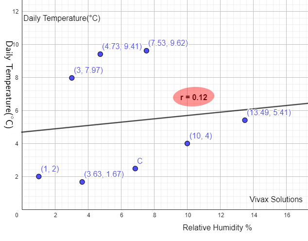
The following graphs shows the relative humidity and daily temperature of a European village for 8 days. The product moment correlation coefficient is 0.12. Carry out a hypothesis test at 5% significance level.

 

From the above table,
Significance level = 5% | sample size = 8
In null hypothesis, we assume that there is no correlation between the data, until it is proven otherwise.
H₀: ρ = 0 | H₁: ρ > 0 Test statistic, r = 0.12
Critical value = 0.6215
Since r < 0.6215, the critical value, a significance event has happened. That means the calculated value of r is in the critical region. There is evidence to reject the null hypothesis and we accept the alternative hypothesis.That means, there is correlation between humidity and temperature in this particular village.

E.g.2

A survey was conducted in 15 households to check the correlation between monthly gas bill and temperature. The PMCC of the data is 0.12. Carry out a hypothesis test at 5% significance level to see whether there is a correlation between the two sets of data.

 

From the above table,
Significance level = 5% | sample size = 15
Since this is a two-tailed test, the significance level is halved for each critical region.
H₀: ρ = 0 | H₁: ρ > 0 Test statistic, r = 0.12
Critical valueS = ± 0.514
Since r < 0.514, the critical value, a significant thing event has happened. That means the calculated value of r is in the critical region. There is no evidence to reject the null hypothesis and we accept the null hypothesis.That means, there is a positive correlation between the gas bill and temperature.

E.g.3

Dave thinks there is no correlation between the number of hours that 14-year-olds spend their time on studies and their corresponding IQ levels. He chose 8 students in his class and calculated the PMCC, r, for the set of data. The data is as follows:

Study Hours	1	2	3	4	5	6	7	8
IQ	101	102	105	104	120	103	120	108

PMCC, r = 0.5515
Carry out a one-tailed hypothesis test at 10% significance level.
H₀: ρ = 0 | H₁: r> 0 Test statistic, r = 0.5515
Critical valueS = 0.5067
Since r > 0.5067, the critical value, a significant event has not happened. That means, the value of PMCC - r or the test statistic - is not in the critical region. There is no evidence to reject the null hypothesis and we accept the null hypothesis.That means, there is no correlation between the number of study hours and the IQ of students.

Hypothesis Testing with Normal Distribution

If a continuous variable can be modeled by the Normal Distribution, we can use a sample statistic to test a population parameter.
E.g. mean of the population

Population: X ~ N(µ, σ²) | Sample: X̄~ N(µ, σ²/n)

The variance or square of the standard deviation of the sample, however, must be divided by the size of the sample, when used for a sample mean.

E.g.1

The management of a supermarket suspect that the mass of sliced bread of a certain brand is less than 500g, as shown on the wrapper.They have found out that the mass of bread is normally distributed with a standard deviation of 20g. They took a sample of 25 loves of bread and found out that the mean mass was 493g. Carry out a hypothesis test at 5% significance level to check that the loaves are under-weight.

Since the company is checking whether the mass is less, the two hypotheses take the following form:
H₀: µ = 500 | H₁: µ < 500
Population: X ~ N(µ, σ²)| X̄ ~ N(µ, σ²/n)
On the basis of null hypothesis: X̄ ~ N(500, 400/25)
X̄ ~ N(500, 4²)
The test statistics is 493
P(X̄ < 493) = 0.0401 < 0.05
Since the test statistic falls into the critical region, a significant event has occurred. There is sufficient evidence to reject the null hypothesis and accept the alternate hypothesis.That means the mass of the bread in the particular brand is less than 500g that it has been claimed to be.

E.g.2

A manufacturer claims that the average lifespan of their light bulbs is 1500 hours. A random sample of 50 light bulbs is tested, and the sample mean lifespan is found to be 1480 hours with a standard deviation of 100 hours. At 5% significance level, conduct a hypothesis test to test manufacture's claim.

Since the testing involves whether the actual life span is less than the claim, the two hypotheses take the following form:
H₀: µ = 1500 | H₁: µ < 1500
Population: X ~ N(µ, σ²)| X̄ ~ N(µ, σ²/n)
On the basis of null hypothesis: X̄ ~ N(1500, 100²/50)
X̄ ~ N(1500, 14.14²)
The test statistic is 1480
P(X̄ < 1450) = 0.078 > 0.05
Since the test statistic does not fall into the critical region, a significant event has not occurred. There is insufficient evidence to reject the null hypothesis and hence it is accepted.That means the the lifespan of light bulbs is 1500 hours.

E.g.3

A major electric car manufacturer claims that its new electric vehicle model has an average range of 400 miles on a single charge. A random sample of 36 vehicles has been chosen to be tested. If the standard deviation of the range is 18 miles, find the critical values for a hypothesis test at 1% significance level.

Since the testing involves finding the critical values:
H₀: µ = 400 | H₁: µ ≠ 400
Population: X ~ N(µ, σ²)| X̄ ~ N(µ, σ²/n)
On the basis of null hypothesis: X̄ ~ N(400, 18²/36)
X̄ ~ N(400, 3²)
In order to find the critical values, we can use the standard normal distribution.
Z ~ N(0, 1²)
Z = (X̄ - µ)/σ
For a two-tailed test, the significance level is halved for the two ends of the normal distribution - 0.5% at each end.
z such that P(Z < z) = 0.005 must be found.
Φ(z) = 0.005
z = Φ^-1(0.005)
= -2.56
Z = (X̄ - µ)/σ → -2.56 = (X̄ - 400)/3
X̄ = 392.32
z such that P(Z > z) = 0.005 must be found.
Φ(z) = 0.005
z = Φ^-1(0.005)
= 2.56
Z = (X̄ - µ)/σ → 2.56 = (X̄ - 400)/3
X̄ = 407.68
The critical region: X̄ > 407.68 or X̄ or X̄ < 392.32

E.g.4

Quitts, a brewery, claims that the alcohol content of its flagship beer is 5.0% ABV (Alcohol By Volume). A random sample of 35 bottles is tested, and the sample mean alcohol content is found to be 5.12% ABV with a standard deviation of 0.15% ABV. Test the brewery's claim at 1% significance level. Determine the critical values for this test.

H₀: µ = 5.0 | H₁: µ > 5.0
Population: X ~ N(µ, σ²)| X̄ ~ N(µ, σ²/n)
On the basis of null hypothesis: X̄ ~ N(5, 0.025²)
X̄ ~ N(500, 0.025²)
The test statistics is 5.12
P(X̄ > 5.06) = 0.0082 < 0.01
Since the test statistic falls into the critical region, a significant event has occurred. There is sufficient evidence to reject the null hypothesis and accept the alternate hypothesis.That means the the alcohol content in beer produced by Quitts is higher than the claim made by the company for the same.
In order to find the critical value, the following procedure is used:
H₀: µ = 5.0 | H₁: µ > 5.0
Population: X ~ N(µ, σ²)| X̄ ~ N(µ, σ²/n)
On the basis of null hypothesis: X̄ ~ N(5, 0.025²)
X̄ ~ N(5, 0.025²)
The
In order to find the critical values, we can use the standard normal distribution.
Z ~ N(0, 1²)
Z = (X̄ - µ)/σ
For a one-tailed test, the significance level at 1%,
z such that P(Z > z) = 0.01 must be found.
Φ(z) = 0.01
z = Φ^-1(0.01)
= 5.06
Z = (X̄ - µ)/σ → 5.06 = (X̄ - 5)/0.025
X̄ = 5.13
The critical region: X̄ > 5.13%

 

You will find the following tutorials useful too: